We are often asked what programs can view DIRSIG's image outputs and how to import the raw DIRSIG image data files into other tools for further processing.
For basic image viewing, DIRSIG-4.4.0 now includes a very simple viewing tool. Launch it from the main simulation editor window by selecting the "Start image viewer" option from the "Tools" menu.
If you run your simulation from the GUI simulation editor, new image files are automatically added to the list in the image viewer as they are generated. If you want to manually add files to the list, simply select the "Open" item from the "File" menu or the toolbar.

If you run your simulation from the GUI simulation editor, new image files are automatically added to the list in the image viewer as they are generated. If you want to manually add files to the list, simply select the "Open" item from the "File" menu or the toolbar.
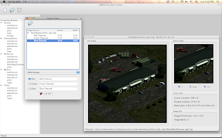
Here is a screenshot of the main image viewer window. The top part contains the list of currently opened files and the bands within those image files.
 To view a single band as a gray-scale image, choose "Single Band Display" from the combo box and then click on the image band that you want. Finally, click "Load Band".
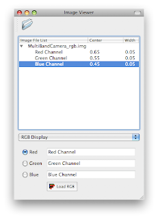
You can also load three bands at once. One band will be visualized in red, another in green, and the last in blue. Choose "RGB Display" from the combo box. Then, in sequence, click the radio button next to each color followed by the band that you want. Finally, click "Load RGB".
Note that you can use this to view simulated color images. Assign the Red Channel from DIRSIG to the Red color, the Green Channel to the Green, etc. Also note that you are not limited to this. You can assign arbitrary bands to arbitrary colors. This lets you reproduce visualizations such as false color infrared.
 To view a single band as a gray-scale image, choose "Single Band Display" from the combo box and then click on the image band that you want. Finally, click "Load Band".
You can also load three bands at once. One band will be visualized in red, another in green, and the last in blue. Choose "RGB Display" from the combo box. Then, in sequence, click the radio button next to each color followed by the band that you want. Finally, click "Load RGB".
Note that you can use this to view simulated color images. Assign the Red Channel from DIRSIG to the Red color, the Green Channel to the Green, etc. Also note that you are not limited to this. You can assign arbitrary bands to arbitrary colors. This lets you reproduce visualizations such as false color infrared.

The right side of the image window has a "Zoom Image" view of the image. You can control the zoom factor using the "In", "Out" and "Reset" buttons below it. Clicking your left mouse button inside either the "Zoom Image" or "Full Image" regions will center the zoomed area where you clicked. The panels below provided some live feedback of the raw data associated with the pixel your mouse is currently over.
The full image can be saved (for use in a presentation, etc.) to a PNG, JPG, etc. by selecting the "Save As" option from the "File" menu.
If the image file has more than one band, the "Spectral Plot" window can be opened. The "Spectral Plot" window displays a plot of the current pixel across all the bands in the image file.
The built-in Image Viewer tool is very primitive and is only intended for quick visualization. For real image exploitation, here are a few of the options available to you:
For programmers, it is not difficult to write (or find an existing) parser for these image files. DIRSIG uses the ENVI image format, which consists of two separate files: a binary image data file and an ASCII/Text image header file. The binary image data is written in native endian (byte-order) as double precision radiances in a band-interleaved by pixel ordering with no additional headers/offsets in the binary image file. This binary image data file is typically created with a ".img" file extension, but the user can change this extension in their simulation configuration.
For programmers, it is not difficult to write (or find an existing) parser for these image files. DIRSIG uses the ENVI image format, which consists of two separate files: a binary image data file and an ASCII/Text image header file. The binary image data is written in native endian (byte-order) as double precision radiances in a band-interleaved by pixel ordering with no additional headers/offsets in the binary image file. This binary image data file is typically created with a ".img" file extension, but the user can change this extension in their simulation configuration.
In addition to the binary image data file, DIRSIG automatically creates an ENVI Image Header file, which typically has a ".img.hdr" file extension. This header file is simply an ASCII/Text description of the format for the binary image data file. If you explore that image header file, you can find all the critical information needed to read the image data file into most data processing environments. For Matlab programmers, check out these MATLAB scripts to read ENVI image data files. For the C and C++ programmers, check out the GDAL library for parsing raster, geospatial data formats.
Comments