One of the new features that will be in the upcoming DIRSIG 4.4.2 release is something that we have been calling "data-driven focal planes". This mechanism had been on the drawing board for many years and we finally had a reason to implement it on our contract to help model the Landsat Data Continuity Mission (LDCM) sensors, or what many of you will come to know as Landsat 8 when it is launched in December 2012. The concept of the "data-driven" focal plane was to provide an alternative to the parameterized detector array geometry, where you specify the focal length, the number of pixels, the pixel pitch and pixel spacings. Instead a "data-driven" focal plane uses a "database" where each record describes both the geometric and radiometric properties of a single pixel. The key feature is that the geometric and optical properties are described at the front of the aperture. This allows the model to ingest optical predictions from complex optical model packages like Code V, Oslo, etc. or to use measurements captured during calibration of real hardware.
On the LDCM project, we are using measurements of the pixels projected through the entire optical system. The geometric measurements capture all of the distortions imparted by the optical path and any alignment present in the assembly of the focal plane models (we should emphasize that both the reflective and thermal instruments are excellent instruments with minimal distortions and alignment errors). In addition to the geometric location of each pixel, the calibration procedures captured many key radiometric features including variations in the spectral response, gain, and noise across the focal planes. This new data-driven mechanism allows as much (or as little) data to be directly described to DIRSIG on a per-pixel basis.
As valuable as this feature is for assisting in the creation of very precise simulations of actual instruments, the mechanism is also useful for modeling Color Filter Arrays (CFAs). There have been frequent requests over the years for the ability to model a Bayer Pattern focal plane. The Bayer pattern was developed as a method to capture red, green and blue imagery using a single array. The technique would fall under the modern definition of "compressive sensing" because the key idea was that rather than each pixel trying to capture all three colors, each pixel would capture a single color and the remaining two colors would be interpolated from adjacent pixels capturing the other colors (see images below, courtesy of Wikipedia):


Although the Bayer pattern is just one of many CFA patterns that have been developed over the years, it is one of the most popular and is featured in many consumer imaging systems including most point-and-shoot cameras, mobile phone cameras, etc. The data-driven focal plane mechanism provides an easy way to model any CFA focal plane because it allows the user to specify the spectral response of every pixel.
Making the Pixel Database
The first thing we need is a pixel database that describes (for each pixel):
The first two columns are the X and Y coordinates of the pixel, which were included for human bookkeeping purposes only (later we will instruct the DIRSIG model to ignore these two fields). The next two columns are the X and Y angles of the pixel pointing direction, which were computed using from the arctangent of the focal length and the physical location of the pixel. The next two columns are the X and Y IFOVs, which were computed from the arctangent of the focal length and the pixel size. The last column is the index of the spectral response curve to use for this pixel.
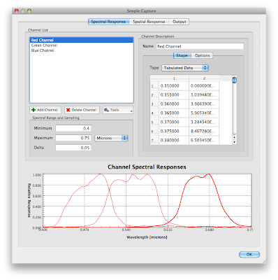
Importing the Filter Responses
The image below shows the red, green and blue pixels that were imported into the platform model using one of the various import mechanisms available. The channel indexes in the pixel database files refer to the curves in this list starting at 0. Hence, 0 maps to red, 1 to green and 2 to blue. Referring back to the pixel database, you can see that the first row of pixels is a Red/Green row (with channel indexes alternating between 0 and 1) and the last row is a Blue/Green row (with channel indexes alternating between 1 and 2):
Using Attribute Fields
Although the pixel X/Y coordinates in our pixel file are not going to be used by the model, the pixel database supports a user-defined number of "attribute" columns before the geometric and radiometric description begins (pixel angles, pixel IFOVs, etc.). When we supply the pixel database to DIRSIG, we need to tell it that there are "2" attribute fields in our file so it can correctly skip them and extract the geometric and radiometric description for the pixel. You might be asking yourself "If DIRSIG is going to skip them, what is the point in including them at all?" The answer to that question is that DIRSIG allows you to use those fields to sub-select some set of pixels from the file. The utility of this selection mechanism is beyond the scope of this article, but one example is how we have been modeling the LDCM focal planes. The LDCM pixel database includes attribute fields that indicate which band, which focal plane model and which "set" (the LDCM focal planes have backup pixels) the pixel belongs to. This has allowed us to simulate using the backup set of pixels for a given focal plane module using a simple run-time selection rule.
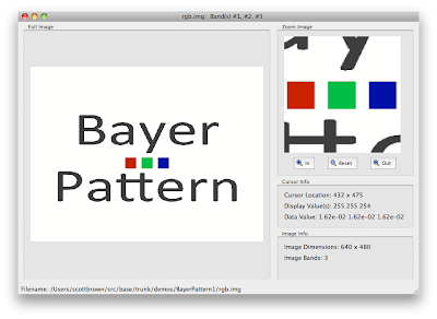
Example Scene
We created a special scene that would demonstrate the collection behavior of this type of sensor. The image below (click to see the larger version) shows the scene imaged with a true RGB, 3 focal plane camera (separate focal planes for red, green and blue). The sharp edges of the high contrast black and white text and color panels will stress the intrapolation scheme used to estimate the missing colors in pixels near these edges when imaged with the Bayer pattern focal plane.
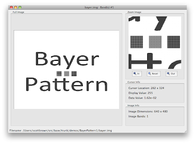
Raw Bayer Pattern Image
The image below (click to see the larger version) is the raw radiance image from the Bayer pattern focal plane. Note that that it is not a color image at this point because the image contains red, green and blue data mosaiced within the single band image. The zoom of the center area containing the color panels makes the filter pattern of the pixels apparent. To turn this into a real color image, an algorithm to demosaic the color information from neighboring pixels must be applied to this raw data.
Demosaicing the Bayer Pattern Image
To demosaic the color information and create an RGB image, a simple program was written. It implements a very simple bi-linear interpolation approach to estimate the other colors in a given pixel (a good survey of demosaic algorithms for Bayer Pattern focal planes can be found here). The resulting RGB image is shown below:

If you zoom into the high contrast edges of the letters you can see the artifacts from the demosaicing process. A better algorithm would make a nicer image, but you get the point.

Summary
The goal of this article was to introduce you to the new data-driven focal plane mechanism that will appear in DIRSIG 4.4.2 and to demonstrate it with a color filter array focal plane example. Note that although this example focused on the 3-color Bayer pattern, any pattern with any number of filters can be modeled using this approach. This example will appear in DIRSIG 4.4.2 as a new demonstration.
On the LDCM project, we are using measurements of the pixels projected through the entire optical system. The geometric measurements capture all of the distortions imparted by the optical path and any alignment present in the assembly of the focal plane models (we should emphasize that both the reflective and thermal instruments are excellent instruments with minimal distortions and alignment errors). In addition to the geometric location of each pixel, the calibration procedures captured many key radiometric features including variations in the spectral response, gain, and noise across the focal planes. This new data-driven mechanism allows as much (or as little) data to be directly described to DIRSIG on a per-pixel basis.
As valuable as this feature is for assisting in the creation of very precise simulations of actual instruments, the mechanism is also useful for modeling Color Filter Arrays (CFAs). There have been frequent requests over the years for the ability to model a Bayer Pattern focal plane. The Bayer pattern was developed as a method to capture red, green and blue imagery using a single array. The technique would fall under the modern definition of "compressive sensing" because the key idea was that rather than each pixel trying to capture all three colors, each pixel would capture a single color and the remaining two colors would be interpolated from adjacent pixels capturing the other colors (see images below, courtesy of Wikipedia):
Although the Bayer pattern is just one of many CFA patterns that have been developed over the years, it is one of the most popular and is featured in many consumer imaging systems including most point-and-shoot cameras, mobile phone cameras, etc. The data-driven focal plane mechanism provides an easy way to model any CFA focal plane because it allows the user to specify the spectral response of every pixel.
Making the Pixel Database
The first thing we need is a pixel database that describes (for each pixel):
- The pointing direction of pixel as an X/Y angle relative to the optical axis
- The angular instantaneous field-of-view (IFOV) in the X/Y dimensions
- The index of the spectral response to use in the channel response list
1 0 -0.0637136 -0.0479632 0.0002 0.0002 1
2 0 -0.0635145 -0.0479632 0.0002 0.0002 0
3 0 -0.0633153 -0.0479632 0.0002 0.0002 1
4 0 -0.0631161 -0.0479632 0.0002 0.0002 0
...
636 479 0.0631161 0.0477636 0.0002 0.0002 1
637 479 0.0633153 0.0477636 0.0002 0.0002 2
638 479 0.0635145 0.0477636 0.0002 0.0002 1
639 479 0.0637136 0.0477636 0.0002 0.0002 2
The first two columns are the X and Y coordinates of the pixel, which were included for human bookkeeping purposes only (later we will instruct the DIRSIG model to ignore these two fields). The next two columns are the X and Y angles of the pixel pointing direction, which were computed using from the arctangent of the focal length and the physical location of the pixel. The next two columns are the X and Y IFOVs, which were computed from the arctangent of the focal length and the pixel size. The last column is the index of the spectral response curve to use for this pixel.
Importing the Filter Responses
The image below shows the red, green and blue pixels that were imported into the platform model using one of the various import mechanisms available. The channel indexes in the pixel database files refer to the curves in this list starting at 0. Hence, 0 maps to red, 1 to green and 2 to blue. Referring back to the pixel database, you can see that the first row of pixels is a Red/Green row (with channel indexes alternating between 0 and 1) and the last row is a Blue/Green row (with channel indexes alternating between 1 and 2):

Using Attribute Fields
Although the pixel X/Y coordinates in our pixel file are not going to be used by the model, the pixel database supports a user-defined number of "attribute" columns before the geometric and radiometric description begins (pixel angles, pixel IFOVs, etc.). When we supply the pixel database to DIRSIG, we need to tell it that there are "2" attribute fields in our file so it can correctly skip them and extract the geometric and radiometric description for the pixel. You might be asking yourself "If DIRSIG is going to skip them, what is the point in including them at all?" The answer to that question is that DIRSIG allows you to use those fields to sub-select some set of pixels from the file. The utility of this selection mechanism is beyond the scope of this article, but one example is how we have been modeling the LDCM focal planes. The LDCM pixel database includes attribute fields that indicate which band, which focal plane model and which "set" (the LDCM focal planes have backup pixels) the pixel belongs to. This has allowed us to simulate using the backup set of pixels for a given focal plane module using a simple run-time selection rule.
Example Scene
We created a special scene that would demonstrate the collection behavior of this type of sensor. The image below (click to see the larger version) shows the scene imaged with a true RGB, 3 focal plane camera (separate focal planes for red, green and blue). The sharp edges of the high contrast black and white text and color panels will stress the intrapolation scheme used to estimate the missing colors in pixels near these edges when imaged with the Bayer pattern focal plane.

Raw Bayer Pattern Image
The image below (click to see the larger version) is the raw radiance image from the Bayer pattern focal plane. Note that that it is not a color image at this point because the image contains red, green and blue data mosaiced within the single band image. The zoom of the center area containing the color panels makes the filter pattern of the pixels apparent. To turn this into a real color image, an algorithm to demosaic the color information from neighboring pixels must be applied to this raw data.

Demosaicing the Bayer Pattern Image
To demosaic the color information and create an RGB image, a simple program was written. It implements a very simple bi-linear interpolation approach to estimate the other colors in a given pixel (a good survey of demosaic algorithms for Bayer Pattern focal planes can be found here). The resulting RGB image is shown below:

If you zoom into the high contrast edges of the letters you can see the artifacts from the demosaicing process. A better algorithm would make a nicer image, but you get the point.

Summary
The goal of this article was to introduce you to the new data-driven focal plane mechanism that will appear in DIRSIG 4.4.2 and to demonstrate it with a color filter array focal plane example. Note that although this example focused on the 3-color Bayer pattern, any pattern with any number of filters can be modeled using this approach. This example will appear in DIRSIG 4.4.2 as a new demonstration.
Comments